main

In [1]:

import os
from omegaconf import OmegaConf
import pandas as pd
import numpy as np
import rasterio as rio
import matplotlib.pyplot as plt
import geopandas as gpd
import seaborn as sns
from tqdm.notebook import tqdm
#
from IPython.display import IFrame, Image
#
from src import utils as ut
from src import geo
from src import data
from src import plot
%matplotlib widget
%load_ext autoreload
%autoreload 2

Main task:

starting from a peak in an Italian region, create a visibility network of mountain peaks and identify a series of routes with the best panoramic views Digital elevation model (DEM) of the whole Italian territory https://tinitaly.pi.ingv.it/

Environment Setup

set random seeds and create initial directories if not existing

In [2]:

conf = OmegaConf.load("config.yaml")
ut.set_environment(conf.env.seed)
os.makedirs(conf.env.figures.path, exist_ok=True)

Data retrieval

download required data

Name	Author	CRS	EPSG	License
TINITALY 1.1 Digital Elevation Model	INGV Tarquini et al.	WGS84 UTM zone 32N	32062	CC BY 4.0
ISTAT Italian boundaries	ISTAT	WGS84 UTM zone 32N	32062	CC BY 3.0
SAT Trentino mountain trails	SAT	ETRS89 UTM zone 32N	25832	ODbL

references:

Tarquini, S., Isola, I., Favalli, M., & Battistini, A. (2007). TINITALY, a digital elevation model of Italy with a 10 meters cell size (Version 1.1). Istituto Nazionale Di Geofisica e Vulcanologia (INGV), 10. https://doi.org/10.13127/tinitaly/1.1
Tarquini, S., Isola, I., Favalli, M., Mazzarini, F., Bisson, M., Pareschi, M. T., & Boschi, E. (2007). TINITALY/01: A new triangular irregular network of Italy. Annals of Geophysics. https://doi.org/10.4401/ag-4424
Istituto Nazionale di Statistica. (2023). Confini delle unità amministrative a fini statistici al 1° gennaio 2023. https://www.istat.it/it/archivio/222527
Società degli Alpinisti Tridentini (SAT). (2023). Sentieri dell’intera rete SAT. https://sentieri.sat.tn.it/static/download-sentieri.html

In [3]:

if conf.dem.download:
    data.download_dem(
        url_root     = conf.dem.url.root,
        url_download = conf.dem.url.download,
        outpath      = conf.dem.path,
        tiles        = conf.dem.tiles)
#
if conf.boundaries.download:
    data.download_zip(
        url     = conf.boundaries.url,
        outpath = conf.boundaries.path.root)
#
if conf.routes.download:
    data.download_zip(
        url     = conf.routes.url,
        outpath = conf.routes.path)

Data Exploration

DEM Raster

Check rasters metadata for validation

In [4]:

In [4]:

Table 1: Metadata of the downloaded DEM tiles.

	CRS	Shape	Height [km]	Width [km]
Tile
w51560	EPSG:32632	(5005, 5010)	50.05	50.1
w51060	EPSG:32632	(5010, 5010)	50.10	50.1
w50560	EPSG:32632	(5010, 5010)	50.10	50.1
w51565	EPSG:32632	(5010, 5010)	50.10	50.1
w51065	EPSG:32632	(5010, 5010)	50.10	50.1
w50565	EPSG:32632	(5010, 5010)	50.10	50.1
w51570	EPSG:32632	(5010, 5010)	50.10	50.1
w51070	EPSG:32632	(5010, 5010)	50.10	50.1
w50570	EPSG:32632	(5010, 5010)	50.10	50.1

some tiles have different shapes as they are at the boundaries of Italy.

Italian Boundaries

In [5]:

reg = gpd.read_file(os.path.join(conf.boundaries.path.root, conf.boundaries.path.shp))

In [6]:

Code

reg = gpd.read_file(os.path.join(conf.boundaries.path.root, conf.boundaries.path.shp))
print("COLUMNS: " + str(reg.columns))
print("CRS: " + str(reg.crs))

COLUMNS: Index(['COD_RIP', 'COD_REG', 'COD_PROV', 'COD_CM', 'COD_UTS', 'DEN_PROV',
       'DEN_CM', 'DEN_UTS', 'SIGLA', 'TIPO_UTS', 'Shape_Area', 'geometry'],
      dtype='object')
CRS: EPSG:32632

columns are described here: https://www.istat.it/it/files//2018/10/Descrizione-dei-dati-geografici-2020-03-19.pdf

Filter out for the desired region of interest by looking at the field DEN_UTS (or DEN_PROV) for the Provincia Autonoma di Trento. Switch it to COD_REG if interested in a region.

In [7]:

Code

reg = reg.loc[reg.DEN_UTS.str.lower().str.contains(str(conf.boundaries.region).lower())]
reg

	COD_RIP	COD_REG	COD_PROV	COD_CM	COD_UTS	DEN_PROV	DEN_CM	DEN_UTS	SIGLA	TIPO_UTS	Shape_Area	geometry
21	2	4	22	0	22	Trento	-	Trento	TN	Provincia autonoma	6.208170e+09	POLYGON ((716676.337 5153931.623, 716029.354 5...

Routes

In [8]:

Code

routes = gpd.read_file(conf.routes.path)
print("COLUMNS: " + str(routes.columns))
print("CRS: " + str(routes.crs))

COLUMNS: Index(['numero', 'competenza', 'denominaz', 'difficolta', 'loc_inizio',
       'loc_fine', 'quota_iniz', 'quota_fine', 'quota_min', 'quota_max',
       'lun_planim', 'lun_inclin', 't_andata', 't_ritorno', 'gr_mont',
       'comuni_toc', 'geometry'],
      dtype='object')
CRS: EPSG:25832

This needs to be converted to the WGS84 - UTM 32N

Check the amount of errors between the nominal planimetric length of the routes (lun_planim), and the one computed by geopandas.

In [9]:

routes['error'] = routes.geometry.length-routes.lun_planim

Explore the distributions of the routes metadata

In [10]:

px = 1/plt.rcParams['figure.dpi']
fig, ax = plt.subplots(figsize=(conf.env.figures.width*px,conf.env.figures.width*px*0.5))
routes.plot(kind='box', subplots=True, sharey=False, widths=0.5, ax=ax,
            title='Routes information distribution')
plt.subplots_adjust(wspace=1.3)
fpath = os.path.join(conf.env.figures.path, "fig-routes-dst.png")
plt.savefig(fpath)
plt.close()
Image(fpath, width=conf.env.figures.width, height=conf.env.figures.width*0.5)

/home/davide/.local/share/virtualenvs/unitn_geospatial-7KxAb5oA/lib/python3.11/site-packages/geopandas/plotting.py:982: UserWarning: To output multiple subplots, the figure containing the passed axes is being cleared.
  return PlotAccessor(data)(kind=kind, **kwargs)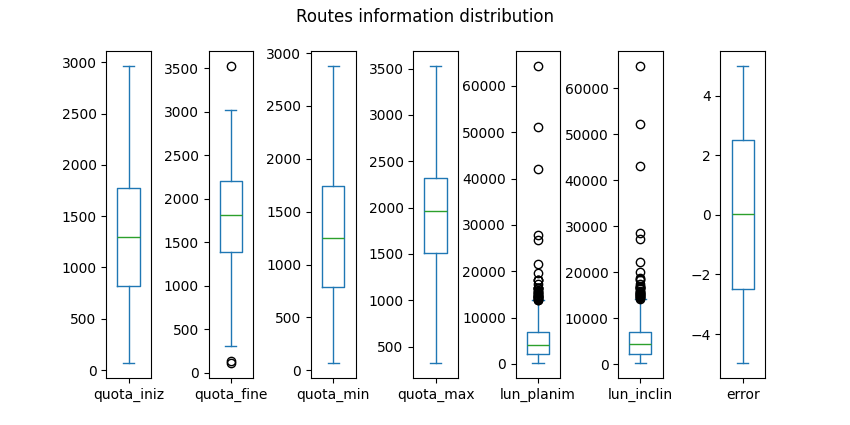

Figure 1: Distribution of the quantitative columns of the routes shapefile.

Visualize if some routes are out of the regional bounds

In [11]:

raster = data.merge_rasters(conf.dem.path, conf.dem.tiles, resolution=conf.dem.downsampling)
routes = routes.to_crs(raster.rio.crs)
routes = data.add_raster_coords(routes, raster.rio.transform)
reg = data.add_raster_coords(reg, raster.rio.transform, area=True)
fig = plot.plot_routes_bounds(np.array(raster[0]), reg, routes)
fpath = os.path.join(conf.env.figures.path, "fig-routes-out.html")
fig.write_html(fpath)
IFrame(src=fpath, width=conf.env.figures.width, height=conf.env.figures.width*0.84)

Figure 2: Exploratory analysis of in- and out-of-bounds routes.

Data Preprocessing

In [12]:

if conf.env.prepare_data:
    # Merge tiles into unique raster and downsample
    raster = data.merge_rasters(conf.dem.path, conf.dem.tiles, resolution=conf.dem.downsampling)
    # Get regional (provincial) boundaries
    reg = gpd.read_file(os.path.join(conf.boundaries.path.root, conf.boundaries.path.shp))
    reg = reg.to_crs(raster.rio.crs)
    reg = reg.loc[reg.DEN_UTS.str.lower().str.contains(str(conf.boundaries.region).lower())]
    # Clip raster to region boundaries
    # raster = raster.rio.clip(reg.geometry.values, reg.crs)
    # Save raster
    raster.rio.to_raster(conf.dem.output)
    # Routes preparation
    routes = gpd.read_file(conf.routes.path)
    routes = routes.to_crs(raster.rio.crs)
    # Extract rows and columns coordinates of each point in the line
    routes['coords'] = routes['geometry'].apply(lambda x: x.coords.xy)
    routes['row'], routes['col'] = zip(*routes['coords'].apply(
        lambda x: rio.transform.rowcol(raster.rio.transform(), x[0], x[1])))
    routes = routes.drop(['coords'], axis=1)
    # Do the same for the region
    reg['coords'] = reg['geometry'].apply(lambda x: x.boundary.coords.xy)
    reg['row'], reg['col'] = zip(*reg['coords'].apply(
        lambda x: rio.transform.rowcol(raster.rio.transform(), x[0], x[1])))
    reg = reg.drop(['coords'], axis=1)
    # Take routes only inside region of interest
    routes = routes[routes.within(reg.geometry.values[0])]
    routes.to_parquet(conf.routes.output)
    reg.to_parquet(conf.boundaries.output)

NOTE: routes modified dataset must be released under ODbL!

In [13]:

raster = rio.open(conf.dem.output)
dem = raster.read(1)
transform = raster.transform
crs = raster.crs
routes = gpd.read_parquet(conf.routes.output)
reg = gpd.read_parquet(conf.boundaries.output)

In [14]:

# #| label: fig-routes-proc
# #| fig-cap: "Exploratory analysis of in- and out-of-bounds routes."
fig = plot.plot_routes_processed(dem, reg, routes)
fpath = os.path.join(conf.env.figures.path, "fig-routes-proc.html")
fig.write_html(fpath)
IFrame(src=fpath, width=conf.env.figures.width, height=conf.env.figures.width*0.84)

Peaks detection

In [15]:

fig = plot.plot_peaks_compare(dem, reg, transform, crs, sizes=[10,50], thresholds=[1000, 2500], )
fpath = os.path.join(conf.env.figures.path, "fig-compare.html")
fig.write_html(fpath)
IFrame(src=fpath, width=conf.env.figures.width, height=conf.env.figures.width*1)

Figure 3: Comparison of the peaks detection procedure with different parameters

organize peaks and metadata inside a geodataframe: * longitude and latitude * raster row and column * peaks names (OSM Overpass API lookup) * check if inside region of interest

In [16]:

peaks_ix, peaks_values = geo.find_peaks(dem, size=conf.peaks.size, threshold=conf.peaks.threshold)
plon, plat = rio.transform.xy(transform, peaks_ix[:, 0], peaks_ix[:, 1], offset='center')
labels = [geo.closest_peak_name(lon, lat, crs) for lon, lat in tqdm(list(zip(plon, plat)))]
#
peaks = gpd.GeoDataFrame(
    data={"row": peaks_ix[:,0], "col": peaks_ix[:,1], "elevation": peaks_values, "name": labels},
    geometry=gpd.points_from_xy(plon, plat, crs=crs), crs=crs)
peaks["inside"] = peaks.geometry.within(reg.geometry.values[0])

In [17]:

In [17]:

Table 2: Computed GeoDataFrame of detected peaks, including georeferences and metadata.

	row	col	elevation	name	geometry	inside
0	0	770	2663.331055	Wetterspitze - Cima del Tempo	POINT (677000.000 5200000.000)	False
1	0	899	2354.733887	Riedspitze - Cima Novale	POINT (689900.000 5200000.000)	False
2	0	1087	2734.199951	Schwarze Riffl - Scoglio Nero	POINT (708700.000 5200000.000)	False
3	0	1202	2503.150879	Speikboden - Monte Spico	POINT (720200.000 5200000.000)	False
4	0	1391	3423.681885	Hochgall - Monte Collalto	POINT (739100.000 5200000.000)	False
...	...	...	...	...	...	...
248	1410	240	1577.568970	Monte Pizzocolo	POINT (624000.000 5059000.000)	False
249	1424	12	1268.843994	Dosso Giallo	POINT (601200.000 5057600.000)	False
250	1457	16	1214.766968	Monte Tecle	POINT (601600.000 5054300.000)	False
251	1495	42	1165.973999	Dosso del Lupo	POINT (604200.000 5050500.000)	False
252	1495	460	1103.145996	None	POINT (646000.000 5050500.000)	False

253 rows × 6 columns

visualize which peaks are inside the region of interest

In [18]:

Figure 4: Labelled mountaintops detected with parameters size=50 and threshold=1000

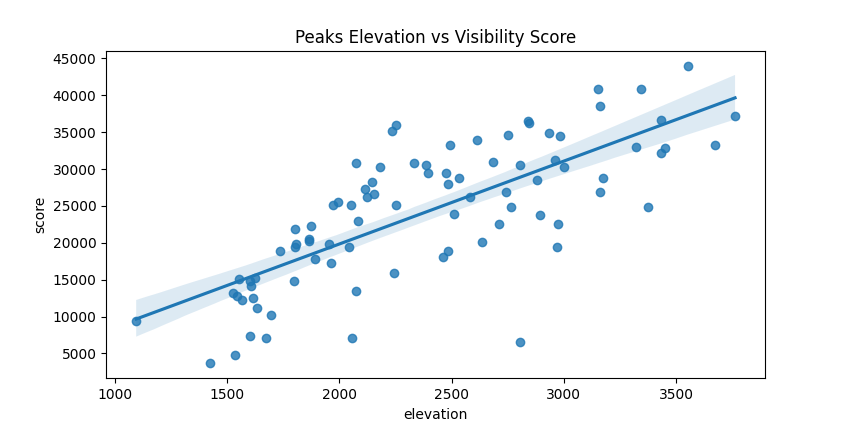
Visibility Network

In [19]:

%%time
G = geo.compute_visibility_network(dem, peaks, crs, transform)

CPU times: user 5.3 s, sys: 250 ms, total: 5.55 s
Wall time: 5.33 s

In [20]:

Figure 5: Peaks Visibility Network showing visibility for each peak. The size of the nodes is their degree, the color is their visibility score.

In [21]:

In [21]:

Table 3: Metadata of the most panoramic mountaintops.

	name	elevation	score
153	Cima Presanella	3551.854004	43982.139194
90	Punta Penia	3342.749023	40791.724952
158	Cima Brenta	3152.949951	40791.724952
162	Cima Tosa	3162.955078	38512.857636
96	Monte Cevedale	3763.043945	37145.537247
165	Anticima di Monte Fumo	3433.218018	36689.763784
108	Cimon del Latemar - Diamantiditurm	2839.964111	36461.877052
155	Cima d'Asta	2843.674072	36233.990321
240	Punta di mezzodì	2253.288086	36006.103589
233	Cima Palon	2232.784912	35094.556663

In [22]:

Figure 6: Correlation visualization between mountaintops elevation and their visibility score.

Routes Visibility Analysis

In [23]:

routes = geo.compute_routes_score(dem, routes, peaks, crs, transform)

In [24]:

routes.columns

Index(['numero', 'competenza', 'denominaz', 'difficolta', 'loc_inizio',
       'loc_fine', 'quota_iniz', 'quota_fine', 'quota_min', 'quota_max',
       'lun_planim', 'lun_inclin', 't_andata', 't_ritorno', 'gr_mont',
       'comuni_toc', 'geometry', 'row', 'col', 'panorama_score_weighted',
       'panorama_score'],
      dtype='object')

In [25]:

In [25]:

Table 4: Metadata of the most panoramic routes.

	numero	denominaz	gr_mont	panorama_score_weighted	competenza	difficolta	loc_inizio	loc_fine	quota_iniz	quota_fine	quota_min	quota_max	lun_planim	lun_inclin	t_andata	t_ritorno	comuni_toc	panorama_score
483	E646	None	MARMOLADA / Colac' - Bufaure - L'Aut	3.862061	SEZ. SAT ALTA VAL DI FASSA	E	VAL DE CONTRIN	pr. FORCIA NEIGRA	1771	2486	1771	2454	2030	2170	02:00	01:30	CANAZEI-CIANACEI	7.821029
95	E207	VIA FERRATA "GIUSEPPE HIPPOLITI"	CIMA DODICI - ORTIGARA	3.447369	SEZ. SAT BORGO VALSUGANA, SEZ. SAT LEVICO	EEA-F	SELLA - località Genzianella	ALTOPIANO	902	1950	902	1970	6480	6780	03:15	02:20	BORGO VALSUGANA, LEVICO TERME	22.345980
297	E157A	SENTIERO "ALBERTO GRESELE"	CARÉGA - PICCOLE DOLOMITI	3.401106	SEZ. SAT VALLARSA	E	MALGA STORTA	QUOTA 1601	1344	1601	1344	1601	1120	1170	00:55	00:30	VALLARSA	3.816173
192	E207A	SENTIERO DELLA GROTTA DI COSTALTA	CIMA DODICI - ORTIGARA	3.089812	SEZ. SAT BORGO VALSUGANA	E	SPIGOLO DI COSTALTA	GROTTA DI COSTALTA	1652	1688	1652	1702	220	240	00:10	00:05	BORGO VALSUGANA	0.689643
420	E322C	None	LAGORAI / Costalta - Croce, LAGORAI / Mànghen ...	2.997636	SEZ. SAT BORGO VALSUGANA	E	MALGA VALSOLÈRO DI SOPRA	PASSO DEL MÀNGHEN	1747	2043	1746	2045	1600	1640	00:50	00:40	TELVE	4.799935

In [26]:

rasterized = rio.features.rasterize(routes.geometry, out_shape=dem.shape,
                                    transform=transform, fill=0)
fig = plot.plot_routes_compare(dem, routes, rasterized)
fpath = os.path.join(conf.env.figures.path, "fig-routes-compare.html")
fig.write_html(fpath)
IFrame(src=fpath, width=conf.env.figures.width, height=conf.env.figures.width*0.6)

Figure 7: Comparison between a raw LineString route (left) from the trails shapefile, and its rasterized version (right).

In [27]:

Figure 8: Labelled mountaintops detected with parameters size=50 and threshold=1000

Project Notebook [main.ipynb]

Environment Setup

Data retrieval

Data Exploration

DEM Raster

Italian Boundaries

Routes

Data Preprocessing

Peaks detection

Visibility Network

Routes Visibility Analysis