Code
conf = OmegaConf.load("config.yaml")
utils.set_environment(conf.env.seed)
os.makedirs(conf.env.figures.path, exist_ok=True)
Davide Calzà

Mat. 238367
davide.calza@studenti.unitn.it
This report outlines a set of procedures for analysing the visibility among mountain peaks and trails in the “Provincia Autonoma di Trento” area, Italy, leveraging on a Digital Elevation Model (DEM). The presented solution aims to identify the mountaintops in the region and compute a Peaks Visibility Network (PVN), which is an undirected graph where nodes represent peaks, and edges indicate mutual visibility. The article provides both an overview of the most connected mountaintops, and a ranking of the most panoramic mountain trails based on a score that measures the visibility between the routes and the peaks. Additionally, it includes a review of existing algorithms and approaches for visibility analysis, along with suggestions for several improvements to enhance the quality and efficiency of the results. This work demonstrates the potential applications of the presented visibility analysis techniques for studying mountaintops. These applications include optimal placement of observation and communication points, historical and military analysis, routing recommender systems, and augmented reality.
Digital Elevation Model, Visibility network, Geospatial analysis, Mountain trails, Mountaintops visibility, Peaks detection

This work is licensed under a Creative Commons Attribution 4.0 International License .
To view a copy of this license, visit
http://creativecommons.org/licenses/by/4.0/
.
Legal Code
Visibility analysis is an important problem in geospatial research, with many applications in the field of Geographic Information Systems (GIS). Digital Elevation Models (DEM) are a commonly used representation of terrain elevation, often provided in a raster format. Each cell in the DEM represents the elevation of the terrain at that point. Several algorithms and approaches have been proposed in the literature[1] to exploit the information contained in the DEM for visibility analysis applications.
One subject area that may find visibility analysis relevant is the study of mountaintops. For example, a visibility network can be computed among mountain peaks to optimally position observation and panoramic points or communication towers. Additionally, topographical information about the mountains and their elevation has historically been crucial for establishing strategic military points. Furthermore, by extending the analysis techniques to mountain trails, it is possible to define a “panoramicity” score, which can be integrated into routing or tourism-oriented recommender systems.
The purpose of this report is to outline procedures for analysing visibility among a set of predefined points. Specifically, given the DEM of a particular region, the aim is to identify mountaintops in the area and establish a visibility network among them. This Peaks Visibility Network (PVN) is an undirected graph where edges connect two nodes (mountaintops) if they are mutually visible. Additionally, this report provides a ranking of the most panoramic mountaintops and mountain trails in the specified region by using the presented visibility analysis techniques. The Region-Of-Interest (ROI) considered for the results presented is the “Provincia Autonoma di Trento” (Trentino), Italy.
The report is structured as follows: Section 2 analyses the state-of-the-art related to the research question. Furthermore, Section 3 provides a description and preliminary overview of the datasets used in the analysis. The proposed solution and results are presented in Section 4, where the procedures adopted for the visibility analysis are described in detail. Finally, Section 5 reports potential future work to integrate the presented solution, and conclusions are drawn in Section 6.
The datasets adopted for the presented analysis are open data, hence publicly available. Overall, three public sources are accessed (Table 1). Access, exploration and preprocessing of the datasets are described in Section 4.
TINITALY 1.1 is an improved Digital Elevation Model (DEM) provided by the Istituto Nazionale di Geofisica e Vulcanologia (INGV)[7,8]. It covers the entire Italian surface with a resolution of 10 metres. The authors propose a Triangular Irregular Network (TIN) DEM format, as it revealed to be the most accurate in relation to the density of the input data. The elevation data was retrieved from multiple sources, such as the Italian regional topographic maps, satellite-based GPS points, ground-based and radar altimetry data[8]. Additional information can be found in the paper and on the website. The data is available split in multiple tiles, each covering an area of approximately 2500 km\(^2\), in a GeoTIFF format. The adopted Coordinate Reference System is WGS84 - UTM zone 32N (EPSG:32602). The work and the dataset are licensed under the Creative Commons Attribution 4.0 license (CC BY 4.0). This dataset is the core of the visibility analyses, as it contains the necessary terrain elevation data.
The information about the boundaries of the Italian administrative units are retrieved from the public dataset published by the Istituto Nazionale di Statistica (ISTAT)[9]. The dataset was last updated on January 1st, 2023, and is available in two versions: a generalized version (less detailed) and a non-generalized version (more detailed). The data is released in a Shapefile format using the WGS84 - UTM zone 32N (EPSG:32602) Coordinate Reference System. The dataset is licensed under the Creative Commons Attribution 3.0 license (CC BY 3.0). Further information, such as the description of the available data and the columns of the datasets can be found on the ISTAT website. This dataset is required to circumscribe the visibility analyses to a limited region of interest, based on administrative boundaries.
The dataset providing a list of the available mountain trails in the Provincia Autonoma di Trento is released by the Società Alpinisti Tridentini (SAT)[10], that operates to maintain the tracks. The dataset contains about 5500 km of mountain trails in the region. It contains various information about the trails, such as the elevation gain, the estimated time to complete the track and their length. It is released in a Shapefile format using the ETRS89 / UTM zone 32N (EPSG:25832) Coordinate Reference System. The dataset is licensed under the Open Data Commons Open Database License (ODbL). This dataset provides an accurate representation of the available mountain trails in the region. Alternatively, it may be possible to gather information about mountain tracks from other public sources such as OpenStreetMap.
This section outlines all the procedures and analysis used to address the initial research question, including data retrieval, analysis and processing, as well as visibility analysis and results. The entire workflow, from the raw data to the final results is depicted in Figure 1 flowchart. Briefly, the steps necessary to produce the results are: data preprocessing (Section 4.1), mountaintops detection (Section 4.2), visibility analysis of both peaks (Section 4.3) and routes (Section 4.5).
The entire approach was developed with the aim of providing a general-purpose solution in a scalable way, in order to easily extend it to different regions of interest and different data sets. If different data sources are used, a custom plugin can be developed to adapt the new data to the input formats used. The following procedures are intended to be used as a starting point for the building of an efficient pipeline; to this end, for simplicity and for computational efficiency, trivial algorithms are employed. Possible integrations and enhancements of the presented work are reported in Section 5.
The presented work is developed using Python, public datasets and open-source software; it can be handled entirely from a configuration file, which is described in the appendix (Section 7.1). Moreover, a random seed is set for reproducibility. The source code can be found at the following link: gitlab.com/davidecalza/unitn_geospatial.
conf = OmegaConf.load("config.yaml")
utils.set_environment(conf.env.seed)
os.makedirs(conf.env.figures.path, exist_ok=True)flowchart LR
classDef out fill: #ff4081
classDef in stroke: #ffa000
classDef op stroke: #00796b
subgraph SUB_RASTER[<font size=5><b> Routes fa:fa-hiking  ]
%% nodes
R_SHP[(<font size=4><b> Routes .shp)]:::in
R_RASTERIZE((<font size=4><b> rasterize)):::op
R_CLIP((<font size=4><b> routes\nclip)):::op
R_RASTER(<font size=4><b> Routes\nRaster)
%% edges
R_SHP -.-> |<font size=5><b>   fa:fa-draw-polygon  | R_RASTERIZE
R_RASTERIZE --> |<font size=5><b>   fa:fa-table-cells-large  | R_CLIP
R_CLIP --> |<font size=5><b>   fa:fa-scissors  | R_RASTER
end
subgraph PPP[<font size=5><b> Peaks fa:fa-mountain    \n ]
subgraph PRP[<font size=5><b> Preprocessing fa:fa-cogs  ]
subgraph PIP[<font size=4><b> Pipeline fa:fa-list  ]
%% nodes
PP((<font size=4><b> down-\nsample)):::op
M((<font size=4><b> merge)):::op
%% edges
PP --> |<font size=5><b>   fa:fa-minimize  | M
end
%% nodes
D1[(<font size=4><b> DEM tile .tif)]:::in
D2[(<font size=4><b> DEM tile .tif)]:::in
D3[(<font size=4><b> DEM tile .tif)]:::in
%% edges
D1 -.-> |<font size=5><b>   fa:fa-th  | PIP
D2 -.-> |<font size=5><b>   fa:fa-th  | PIP
D3 -.-> |<font size=5><b>   fa:fa-th  | PIP
end
%% nodes
T(<font size=4><b> DEM\nRaster)
P(<font size=4><b> Peaks)
PI(<font size=4><b> In-area\nPeaks)
PD((<font size=4><b> peaks\ndetection)):::op
PC((<font size=4><b> peaks\nclip)):::op
PN((<font size=4><b> peaks\nnaming)):::op
O[(<font size=4><b> OSM API)]:::in
%% edges
PIP --> |<font size=5><b>   fa:fa-object-group  | T
T --> |<font size=5><b>   fa:fa-border-style  | PD
PD --> |<font size=5><b>   fa:fa-search-location  | P
P --> |<font size=5><b>   fa:fa-mountain  | PC
PC --> |<font size=5><b>   fa:fa-scissors  | PI
O -.-> |<font size=5><b>   fa:fa-map-marked-alt  | PN
PN --> |<font size=5><b>   fa:fa-tags  | P
end
subgraph PVA[<font size=5><b> Visibility\nAnalysis fa:fa-project-diagram  ]
%% nodes
x[x\nx]:::hidden
VA((<font size=4><b> Visibility\nAnalysis)):::op
VM(<font size=4><b> Visibility\nMatrix)
PS((<font size=4><b> Panorama\nScoring)):::op
%% edges
x ==> VA
VA --> |<font size=5><b>   fa:fa-binoculars  | VM
VM --> |<font size=5><b>   fa:fa-magnifying-glass-location  | PS
end
%% nodes
B[(<font size=4><b> Boundaries\n.shp)]:::in
BP(((<font size=4><b> <b>Most\nPanoramic\nPeaks<b />))):::out
BR(((<font size=4><b> <b>Most\nPanoramic\nRoutes<b />))):::out
%% edges
B -.-> |<font size=5><b>   fa:fa-earth-europe  | PC & R_CLIP
T --> |<font size=5><b>   fa:fa-layer-group  | PVA
R_RASTER --> |<font size=5><b>   fa:fa-route  | PVA
PI --> |<font size=5><b>   fa:fa-mountain  | PVA
P --> |<font size=5><b>   fa:fa-mountain  | PVA
PVA ==> |<font size=5><b>   fa:fa-mountain-sun  | BP
PVA ==> |<font size=5><b>   fa:fa-hiking  | BR
The preliminary step consists in accessing the data and exploring it. In order to provide a reproducible workflow, the datasets are automatically downloaded. In the case of the ISTAT boundaries and the SAT routes, the access is straightforward, as they are simple archives containing the shapefiles; therefore, they share a common interface (function download_zip in the src/data.py module). On the other hand, as previously mentioned in Section 3, the DEM data is divided into multiple tiles. Since the research question focuses on a well-defined region of interest, it is possible to indicate in the configuration file the only tiles to download, by referencing them with their code (e.g., w51560), without handling the entire dataset. The download process is implemented in the download_dem function and it retrieves the resources endpoints by scraping the TINITALY website.
def download_zip(url: str, outpath: str):
    """download_zip.

    Download a zip file from a given url and extract it to a specified
    output path. The function also disables warnings and verifies the
    SSL context.

    :param url: the url of the zip file to download
    :type  url: str
    :param outpath: the output path where the zip file will be
                    extracted
    :type  outpath: str
    """
    urllib3.disable_warnings()
    os.makedirs(outpath, exist_ok=True)
    ssl._create_default_https_context = ssl._create_unverified_context
    #
    r = requests.get(url, verify=False, timeout=100)
    if r.status_code == 200:
        with zipfile.ZipFile(io.BytesIO(r.content)) as zfile:
            zfile.extractall(outpath)
    else:
ut.excerr(f"Unable to download {url}")def download_dem(
url_root: str,
url_download: str,
outpath: str,
tiles: Union[str, List[str]] = 'all'
):
"""download_dem.
Download and extract Digital Elevation Model (DEM) files from a
given url root and download link.
The function also disables warnings and verifies the SSL context.
This function requires careful handling when downloading from
different website than TINITALY (https://tinitaly.pi.ingv.it/).
:param url_root: the url root of the website that hosts the DEM
files
:type url_root: str
:param url_download: the url download link of the DEM files
:type url_download: str
:param outpath: the output path where the DEM files will be
extracted
:type outpath: str
:param tiles: the codes of the tiles of the DEM files to download
(e.g., ['w51560']), default to 'all'
:type tiles: Union[str, List[str]]
"""
urllib3.disable_warnings()
os.makedirs(outpath, exist_ok=True)
ssl._create_default_https_context = ssl._create_unverified_context
#
with urllib.request.urlopen(
os.path.join(url_root, url_download)
) as response:
soup = BeautifulSoup(response, "html.parser")
urls = []
#
for link in soup.findAll('area'):
end = os.path.join(url_root, link.get('href'))
if tiles == 'all' or np.any([t in end for t in tiles]):
urls.append(end)
for u in tqdm(urls, desc="Downloading DEMs", unit="Tile"):
download_zip(u, outpath)if conf.dem.download:
data.download_dem(
url_root = conf.dem.url.root,
url_download = conf.dem.url.download,
outpath = conf.dem.path,
tiles = conf.dem.tiles)
if conf.boundaries.download:
data.download_zip(
url = conf.boundaries.url,
outpath = conf.boundaries.path.root)
if conf.routes.download:
data.download_zip(
url = conf.routes.url,
outpath = conf.routes.path)A preliminary data exploration phase aims at verifying the congruence of the accessed data and its content. First, all the downloaded DEM tiles are checked to see if they share the same CRS and congruent shapes. Their height and width are also computed from their boundaries coordinates, to check if they are compatible with the declared resolution of 10 metres. Since we are analysing the rasters that are close to the boundaries of Italy, some of them may have different shapes (see Table 2). This is visible also from the TINITALY website[7].
Afterwards, the ISTAT boundaries shapefile is loaded and checked. It provides several columns, with a non-descriptive nomenclature. Since the focus of the research question is to apply analysis on the territory of the “Provincia Autonoma di Trento”, then the shapefile of interest is located in the downloaded folder starting with Prov, and the column of interest is DEN_UTS. Through this column it is possible to access the desired geometry. If the area of interest of the research question was an italian region (e.g., Trentino-Alto Adige), then the correct shapefile would be located in the folder starting with Reg. More information about the structure of the downloaded data and the description of the columns is provided by ISTAT on their website[9].
Similarly, the same exploration is carried out for the SAT routes data. As previously mentioned in Section 3, the routes data is reported in a different CRS than the DEM and the boundaries data. Therefore, in the preprocessing phase, it must be converted for uniformity. The shapefile reports different information about the routes, such as the difficulty levels of the tracks, or elevation gain and length of the trails. Since the length of the routes is also reported, both in terms of planimetry and with inclinations, it may be necessary to verify if they are consistent with the length of the geometry computed by GeoPandas[11]. To this end, an error column is added to the dataframe. The distribution of the quantitative variables is shown in Figure 2. As it is observable, the routes are heterogeneous both in terms of elevations and length. Some routes are longer than 60 km, while others are shorter than 200 metres. This means that careful attention is required in assigning scores to routes, by weighting them in some way based on these parameters. The errors between the nominal length and the computed ones range from -5 to +5 metres; therefore, they can be neglected for this context. Lastly, it may happen that some of the mountain trails maintained by the SAT fall outside the boundaries of the region. This may be a problem in further analysis. Therefore, routes that fall outside the area of interest should be excluded in the preprocessing phase. A representation of the distribution of the routes on the regional area is depicted in Figure 3.
routes['error'] = routes.geometry.length-routes.lun_planim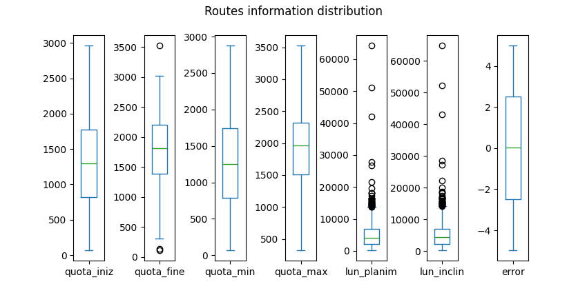
The preprocessing phase is a critical step in the entire analysis, since it allows for data cleaning, uniformity, and rescaling. As shown in Figure 1, the preprocessing phase is divided into two main modules: one for the DEM data, and one for the routes, which compose the two main datasets for the subsequent visibility analysis.
As previously mentioned, DEM data is provided split in different tiles at a resolution of 10 metres. For simplicity and a more efficient computation, each of the downloaded tiles is first downsampled. This operation obviously degrades the quality of the DEM data; therefore, for more accurate analysis, this step may be omitted. The downsampling resolution adopted is 100 metres, and the used resampling technique is the maximum value. This means that the convolution operation for the downsampling takes the maximum value and applies it to the relative cell. This choice was made in order to highlight the most prominent peaks in the region. Subsequently, the downsampled tiles are merged together in one unique raster, in order to ease the further computations. Also this step can be omitted whether parallel processing is integrated, as suggested in Section 2.
In the preliminary development stages, the merged raster was eventually clipped to the regional area. After some analysis it was found that restricting the DEM to the ROI resulted in a strong approximation. This means that peaks were only searched for in the ROI and not outside, with consequences and bias in the final analysis. A consequence of clipping was the generation of not-a-number values in the cells outside the region of interest. This led to two main critical issues: firstly, peaks positioned in the middle of the ROI had higher degrees, i.e. the number of peaks visible from that point, compared to those at the extremes. This was due to the fact that a peak near the edges of the ROI was less likely to have the same degree as a peak in the centre. Secondly, two peaks with an undefined DEM on the trajectory of their line of sight were not considered visible, as the elevation in that area was unknown. It can be assumed that the undefined areas have zero elevation, but this may have been too strong as assumption. For this reason, the entire DEM was retained without clipping, in order to avoid having undefined areas on the lines of sight of the peaks. However, the information about the boundaries of the ROI is necessary to focus the analyses on this specific area. For example, any peak inside the ROI will search for peaks in the entire DEM area provided; on the contrary, peaks outside the DEM will not search for visibility towards other peaks, but will only be used as visibility targets. Therefore, the size of the surrounding DEM should be calibrated according to the needs and the use case.
As regards the routes dataset, it is first converted to the same CRS as the DEM and the boundaries data, i.e., the WGS84 - UTM 32N. As previously mentioned, only those routes that are completely within the ROI are retained. Moreover, two additional variables (row and col) are added for referencing the geometries in terms of rows and columns of their position in the raster to facilitate further analysis. The same operation is applied to the boundaries of the Region of Interest dataset. As aforementioned, the routes dataset is released under the ODbL license; therefore, the processed version of the dataset is also released under the same license.
All the processed datasets are saved locally, in order to be used in the subsequent analysis without requiring to perform the preprocessing procedure again.
if conf.env.prepare_data:
    # Merge tiles into unique raster and downsample
    raster = data.merge_rasters(conf.dem.path, conf.dem.tiles, resolution=conf.dem.downsampling)
    # Get regional (provincial) boundaries
    reg = gpd.read_file(os.path.join(conf.boundaries.path.root, conf.boundaries.path.shp))
    reg = reg.to_crs(raster.rio.crs)
    reg = reg.loc[reg.DEN_UTS.str.lower().str.contains(str(conf.boundaries.region).lower())]
    # Clip raster to region boundaries
    raster = raster.rio.clip(reg.geometry.values, reg.crs)
    # Save raster
    raster.rio.to_raster(conf.dem.output)
    # Routes preparation
    routes = gpd.read_file(conf.routes.path)
    routes = routes.to_crs(raster.rio.crs)
    # Extract rows and columns coordinates of each point in the line
    routes['coords'] = routes['geometry'].apply(lambda x: x.coords.xy)
    routes['row'], routes['col'] = zip(*routes['coords'].apply(
        lambda x: rio.transform.rowcol(raster.rio.transform(), x[0], x[1])))
    routes = routes.drop(['coords'], axis=1)
    # Do the same for the region
    reg['coords'] = reg['geometry'].apply(lambda x: x.boundary.coords.xy)
    reg['row'], reg['col'] = zip(*reg['coords'].apply(
        lambda x: rio.transform.rowcol(raster.rio.transform(), x[0], x[1])))
    reg = reg.drop(['coords'], axis=1)
    # Take routes only inside region of interest
    routes = routes[routes.within(reg.geometry.values[0])]
    routes.to_parquet(conf.routes.output)
reg.to_parquet(conf.boundaries.output)def merge_rasters(
root: str,
tiles: List[str],
resolution: int = 100
) -> xr.DataArray:
"""merge_rasters.
Merge multiple raster files from a given root directory and a list
of tiles. The function also optionally reprojects the rasters to a
specified resolution and resampling method.
Resampling method is set to 'max' by default, meaning that the
maximum value is retained in the rolling windows of the operation.
:param root: the root directory where the raster files are stored
:type root: str
:param tiles: the list of tiles to merge
:type tiles: List[str]
:param resolution: the resampling resolution to reproject the
rasters, default to 100
:type resolution: int
:return: a merged array of the rasters with nodata values set to
np.nan
:rtype: xr.DataArray
"""
rasters = []
for tile in tiles:
t = f'{tile}_s10'
path = os.path.join(root, t, f'{t}.tif')
raster = rxr.open_rasterio(path)
if resolution is not None:
raster = raster.rio.reproject(
raster.rio.crs,
resolution=resolution,
resampling=rio.warp.Resampling.max)
rasters.append(raster)
return merge_arrays(rasters, nodata=np.nan)In order to create a visibility network of the Trentino’s mountaintops, a robust method for the identification of the peaks is required. One possible way consists in getting peaks location from public sources such as OpenStreetMap[12]. This approach allows for human-validated mountaintops locations that are recognised by the community. A second approach consists in inferencing the presence of mountain peaks by exploiting the information contained in the DEM rasters. This mainly allows to detect the presence of peaks also in areas that are scarsely labelled by the community. Moreover, a mountain usually has several peaks, but not all of them are recognised or labelled. As a consequence, secondary peaks may be discarded by using the first approach. Therefore, the approach adopted for the proposed solution relies on the inference from DEM data, providing a scalable and customizable approach for finding mountain peaks.
The implementation of the aforementioned approach is represented by the find_peaks function in the src/geo.py module.
raster = rio.open(conf.dem.output)
dem = raster.read(1)
transform = raster.transform
crs = raster.crs
routes = gpd.read_parquet(conf.routes.output)
reg = gpd.read_parquet(conf.boundaries.output)def find_peaks(
dem: np.ndarray,
size: int,
threshold: float
) -> Tuple[np.ndarray, np.ndarray]:
"""find_peaks.
Find the peaks of a digital elevation model (DEM) array that are
above a given threshold. The function uses a maximum filter to
compare each pixel with its neighbors in a running window of a
given size. The maximum filter returns an array with the maximum
value in the window at each pixel position. The peaks are the
pixels that are equal to the maximum filter output and greater
than the threshold. The function returns the indices and values of
the peaks.
:param dem: the DEM array to find the peaks
:type dem: np.ndarray
:param size: the size of the running window for the maximum filter
:type size: int
:param threshold: the minimum value for the peaks
:type threshold: float
:return: a tuple of the indices and values of the peaks
:rtype: Tuple[np.ndarray, np.ndarray]
"""
filtered = maximum_filter(dem, size)
peaks = (dem == filtered) & (dem > threshold)
indices = np.argwhere(peaks)
values = dem[peaks]
return indices, valuesThis function finds the local maxima in the provided DEM that are larger than a given threshold. It is built on top of the maximum_filter function of the SciPy library[13], which performs a dilation operation on the DEM by replacing each pixel with the maximum value in its neighborhood. The size parameter determines the shape and size of the neighborhood. The function then compares the input DEM with the filtered one, and selects the pixels that are equal, meaning they are not affected by the filtering. These pixels are the local maxima. The function also applies a boolean mask to filter out the maxima that are smaller than the threshold. Therefore, all local maxima below that threshold, i.e., below a certain elevation, are neglected.
As depicted in Figure 4, the tuning of the two parameters offers a scalable approach to the detection of mountaintops. The threshold parameter allows to discard all the detected peaks below a certain elevation; this allows for an elastic customisation of the definition of peaks. Moreover, the size parameter controls the density of the detected peaks. The higher the value, the lower the density of the local maxima, therefore fewer peaks will be detected. On the other hand, if the objective is to find all the peaks, also close to each other, then this parameter should be set to a lower value.
The reported results are produced with size=50 and threshold=1000 (Figure 5), as they revealed to be a reasonable trade-off between the number of peaks detected, their sparsity in space and the computational resources needed for the further analyses, in relation to the topographical properties of the DEM in the ROI.
The detected peaks are then organised into a GeoPandas dataframe (Table 3), where the indexes of the peaks in terms of rows and columns positions in the raster are added (columns row and col). Furthermore, rows and columns are converted into longitude and latitude coordinates in the reference CRS (i.e., WGS82 - UTM zone 32N), in order to form the geometry of the dataframe as points. Additionally, the name of each peak is added as a label column. To retrieve these, an additional function closest_peak_name is provided, with the aim of assigning a recognizable label to each detected peak.
def closest_peak_name(
    lon: float,
    lat: float,
    crs: str,
    around: int = 1000
) -> Optional[str]:
    """closest_peak_name.

    Find the name of the closest natural peak to a given point on a
    map.
    The function:
    1. transforms the longitude and latitude of the point to the
       coordinate reference system (crs) of the map using the
       rio.warp.transform function;
    2. creates an overpy.Overpass object to query the OpenStreetMap
       database;
    3. tries to query the database for the nodes that have the
       natural=peak tag and are within a certain distance (around)
       from the point;
    4. returns the name of the closest node if the query is successful
       and there are nodes found, or None otherwise.

    :param lon: the longitude of the point
    :type  lon: float
    :param lat: the latitude of the point
    :type  lat: float
    :param crs: the coordinate reference system of the map
    :type  crs: str
    :param around: the distance in meters to search for the peaks,
                   default to 1000
    :type  around: int
    :return: the name of the closest peak or None
    :rtype:  Optional[str]
    """
    lon, lat = rio.warp.transform(crs, "EPSG:4326", [lon], [lat])
    #
    api = overpy.Overpass()
    closest = None
    try:
        result = api.query(f"""
            node
              [natural=peak]
              (around: {around}, {lat[0]}, {lon[0]});
            out center tags;
            """)
        nodes = result.nodes
        if len(nodes) > 0:
            closest = nodes[0].tags.get("name", "n/a")
    except:
        pass
    return closest
This function first converts the provided longitude and latitude coordinates of the mountaintop into the WGS 84 (EPSG:4326) CRS, which is the one adopted by OpenStreetMap[14]. By querying the Overpass APIs, which looks up to the OpenStreetMap data, the name of the closest peak (identified with tag natural=peak) in a certain range is retrieved.
The elevation of the detected peak, retrieved from the DEM, is also reported in the geodataframe (column elevation). It is important to highlight that the DEM elevation may not reflect the nominal value of the relative mountaintop, as it depends on how the DEM was generated, and to the resampling method adopted for downsampling the rasters. Another criticality may emerge in case the downsampling resolution is too broad, which may include multiple existing peaks in the single raster cell; in this case, the labelling procedure may be updated to look for the highest peak in the area of the raster cell from the API and use that as a reference, as the resampling method takes the maximum value in the area for the output. Finally, a boolean column named inside is generated, to identify whether the peak is inside the ROI or not.
peaks_ix, peaks_values = geo.find_peaks(dem, size=conf.peaks.size, threshold=conf.peaks.threshold)
plon, plat = rio.transform.xy(transform, peaks_ix[:, 0], peaks_ix[:, 1], offset='center')
labels = [geo.closest_peak_name(lon, lat, crs) for lon, lat in tqdm(list(zip(plon, plat)))]
#
peaks = gpd.GeoDataFrame(
    data={"row": peaks_ix[:,0], "col": peaks_ix[:,1], "elevation": peaks_values, "name": labels},
    geometry=gpd.points_from_xy(plon, plat, crs=crs), crs=crs)
peaks["inside"] = peaks.geometry.within(reg.geometry.values[0])Hover over the scatter points to show labels and elevations for each detected peak.
The proposed Peaks Visibility Network (PVN) consists in a weighted graph representation of the detected peaks. The nodes of the graph represent the peaks, and the edges represent the visibility between them. An edge is created for each pair of peaks if they are considered to be visible to each other. The edges are weighted according to a visibility score based on the inverse of their distance. As the main focus is on the ROI, the visibility between the peaks inside the ROI and all the peaks detected both inside and outside the ROI is checked. This means that the peaks outside the ROI are used exclusively as targets for the visibility score of the peaks inside the ROI. Therefore, the final ranking and results are performed only on the mountaintops inside the ROI. Similar visibility analyses are also performed on the routes within the ROI to provide an overview of the most panoramic mountain trails.
Prior to the computation of the PVN, the definition of visibility was required. In the context of the proposed solution, several assumptions were made:
Possible improvements are described in Section 5. The function is_visible is defined as follows:
@njit
def is_visible(
    dem: np.ndarray,
    peak1: Tuple[int, int],
    peak2: Tuple[int, int],
    tol: float = 0
) -> bool:
    """is_visible.

    Check if two peaks are visible from each other on a digital
    elevation model (DEM) array.
    The function:
    1. uses the bresenham_line function to get the coordinates of the
       line between the two peaks;
    2. computes the sight line as a linear interpolation between the
       heights of the two peaks;
    3. subtracts a tolerance value from the DEM heights along the
       line;
    3. returns True if all the DEM heights are below or equal to the
       sight line, and False otherwise.
    The function is decorated with @njit to speed up the computation
    using Numba.

    :param dem: the DEM array to check the visibility
    :type  dem: np.ndarray
    :param peak1: the coordinates of the first peak as a tuple of
                  (y, x)
    :type  peak1: Tuple[int, int]
    :param peak2: the coordinates of the second peak as a tuple of
                  (y, x)
    :type  peak2: Tuple[int, int]
    :param tol: the tolerance value to subtract from the DEM heights,
                default to 0
    :type  tol: float
    :return: True if the peaks are visible from each other, False
             otherwise
    :rtype:  bool
    """
    y1, x1 = peak1
    y2, x2 = peak2
    z1, z2 = dem[y1, x1], dem[y2, x2]
    y, x = bresenham_line(x1, y1, x2, y2)
    sight = np.linspace(z1, z2, len(x))
    points = np.empty((len(y),), dtype=dem.dtype)
    for i, yi in enumerate(y):
        points[i] = dem[yi, x[i]]-tol
    return np.all(points <= sight)
The procedure identifies the indexes in the raster and the elevations of the two peaks in input. It subsequently applies the Bresenham’s Line algorithm[15] [16], which detects all the raster cells that represent the approximation of a straight line between two cells containing the observed peaks. This version of the algorithm integrates a balancement of the positive and negative errors between x and y coordinates by leveraging an integer incremental error[17].
@njit
def bresenham_line(
    x0: int,
    y0: int,
    x1: int,
    y1: int
) -> Tuple[List[int], List[int]]:
    """bresenham_line.

    Compute the coordinates of a line between two points using the
    Bresenham's algorithm. The function is decorated with @njit to
    speed up the computation using Numba. The function returns a tuple
    of two lists, one for the y-coordinates and one for the
    x-coordinates of the line.
    Reference:
    https://en.wikipedia.org/w/index.php?title=Bresenham%27s_line_algorithm&oldid=1195842736

    :param x0: the x-coordinate of the first point
    :type  x0: int
    :param y0: the y-coordinate of the first point
    :type  y0: int
    :param x1: the x-coordinate of the second point
    :type  x1: int
    :param y1: the y-coordinate of the second point
    :type  y1: int
    :return: a tuple of the y-coordinates and x-coordinates of the
             line
    :rtype: Tuple[List[int], List[int]]
    """
    dx = abs(x1 - x0)
    dy = -abs(y1 - y0)
    sx = 1 if x0 < x1 else -1
    sy = 1 if y0 < y1 else -1
    err = dx + dy
    y, x = [], []
    while True:
        y.append(y0)
        x.append(x0)
        if x0 == x1 and y0 == y1: break
        e2 = err * 2
        if e2 >= dy:
            if x0 == x1: break
            err += dy
            x0 += sx
        if e2 <= dx:
            if y0 == y1: break
            err += dx
            y0 += sy
    return y, x
Afterwards, an array of the size equal to the number of intersected cells is drawn, with values linearly spaced between the elevations of the two peaks, representing the sight line. If all cells between the two peaks cells have elevation values less than their respective point on the sight line, then the two peaks are considered visible. For scalability, the possibility of adding a tolerance to the visibility check is added; however, for the reported results it was not set. A representation is depicted in Figure 6. From the figure, it is possible to highlight another criticality of the provided approach that should be refined: the linearly spaced sight line is an imprecise assumption, therefore it may be refined by spacing the sight points based on the real trajectory of the line. Precisely, the linearly spaced sight points are ideal in the case of a perfect diagonal between two peaks, i.e., the two peaks are on the opposite corners of a squared subgrid in the raster. However, this approximation may result critical primarily in the case of close peaks with a large elevation difference. Reasonably, the higher the resolution of the DEM raster, the more precise will be the representation of the sight line, and more reliable will be the visibility results.

The Peaks Visibility Network (PVN) is an undirected graph with weighted edges. Each detected peak is a node, and is represented by a tuple containing its position in the raster in terms of rows and columns. In this way, it is straightforward to access for further analyses. The edges of the PVN represent the visibility between peaks, with visibility as explained in Section 4.3.1. Formally, the PVN is defined as follows: \[
\text{PVN} = \left\{\begin{matrix}
\mathcal{N} = (y_{p_a}, x_{p_a}) & \forall p_a \in P_a \\
\mathcal{E} = ((y_{p_i}, x_{p_i}), (y_{p_a}, x_{p_a})) & \forall p_i \in P_i, \forall p_a \in P_a, v(p_i, p_a) = T\\
\mathcal{W} = s_{(p_i, p_a)} & \forall (p_i, p_a) \in \mathcal{E}
\end{matrix}\right.
\] where \(\mathcal{N}\), \(\mathcal{E}\), and \(\mathcal{W}\) are respectively the nodes, the edges and the edge weights of the PVN, \(P_a\) is the set of all the detected peaks, both inside and outside the ROI, \(P_i\) is the set of the only detected peaks inside the ROI (\(P_i \subseteq P_a\)), \(v(p_i, p_a)\) is the is_visible function between points \(p_i\) and \(p_a\). The function \(s_{(p_i, p_a)}\) is the visibility score between two peaks, and it is defined later.
In order to assign the edges in an efficient way, a visibility matrix of the peaks is computed. The compute_visibility_matrix is a function that computes a visibility matrix between two sets of coordinates: points1 and points2. A visibility matrix represents the output of the function, with values set to 1 in case of visibility between two points, 0 otherwise. In case the two sets of coordinates were the same, the output matrix would be symmetrical, and with a shape of \(n * n\), where \(n\) is the number of detected peaks. Therefore, in order to improve the efficiency of the procedure, a check is performed on the two sets of coordinates to verify if they are the same. If they are, then only half the matrix will be filled, by avoiding the check of the already processed couples of points. The visibility between a peak and itself (i.e., the diagonal if the matrix is symmetrical) is also set to zero. In the case on the proposed solution, however, the two sets of peaks are different, since the check is performed between the detected peaks inside the ROI (\(P_i\)), and all the peaks detected (\(P_a\)), both inside and outside the ROI. This means the output visibility matrix will be of shape \(n * m\), where \(n\) is the number of detected peaks inside the ROI (\(n = |P_i|\)), and \(m\) is the number of all the detected peaks (\(m = |P_a|\)), with \(n \leq m\).
@njit(parallel=True)
def compute_visibility_matrix(
    dem: np.ndarray,
    points1: np.ndarray,
    points2: np.ndarray
) -> np.ndarray:
    """compute_visibility_matrix.

    Compute the visibility matrix between two sets of points on a
    digital elevation model (DEM) array.
    The function:
    1. uses the is_visible function to check the visibility between
       each pair of points;
    2. returns a boolean matrix with the visibility status of each
       pair of points;
    3. optimizes the computation by skipping the same peak and using
       symmetry if the two sets of points are equal.
    The function is decorated with @njit and parallel=True to speed up
    the computation using Numba.

    :param dem: the DEM array to compute the visibility matrix
    :type  dem: np.ndarray
    :param points1: the first set of points as an array of coordinates
                    (y, x)
    :type  points1: np.ndarray
    :param points2: the second set of points as an array of
                    coordinates (y, x)
    :type  points2: np.ndarray
    :return: the visibility matrix between the two sets of points
    :rtype:  np.ndarray
    """
    visibility = np.zeros((len(points1), len(points2)), dtype=np.bool_)
    eq = points1.shape == points2.shape and (points1==points2).all()
    for i in prange(len(points1)):
        d = i if eq else 0
        for j in prange(d, len(points2)):
            if points1[i][0] == points2[j][0] and points1[i][1] == points2[j][1]:
                continue # skip same peak
            if is_visible(dem, points1[i], points2[j]):
                visibility[i, j] = 1
    return visibility
Once the visibility matrix is computed, the qualitative information about the visibility is obtained. However, the visibility of a mountaintop that is close to the observer may be weighted differently compared to a peak that is more distant. To this end, a visibility score is computed for each edge in the PVN, based on the distance between the pairs of peaks. The visibility score \(s_{(p1,p2)}\) of a pair of peaks \(p1\) and \(p2\) is computed as follows: \[
s_{(p1,p2)} = \frac{1}{1+(w*d_{(p1,p2)}*10^{-3})}
\] where \(d_{(p1,p2)}\) is the distance in metres between the pairs of peaks \(p1\) and \(p2\), and \(w\) is a weight assigned to the distance. This is useful to calibrate the weight of the distance on the final score, depending on the use case. If \(w=0\), then the score is independent of the distance. The function for computing visibility scores is compute_visibility_score, which relies on the function compute_raster_distance for obtaining the distances in metres. The latter transforms the peaks coordinates in terms of rows and columns into a set of coordinates in longitude and latitude. Subsequently, it computes the elementwise distance between the points contained in the lists p1 and p2. Since the CRS of the provided DEM is the “WGS 84 - UTM zone 32N” (EPSG:32632), whose measurement unit is in metres, no further reprojection is needed. Finally, the PVN assigns the computed visibility scores as weights to the edges. This procedure is represented by the function compute_visibility_network.
def compute_visibility_scores(
    p1: np.ndarray,
    p2: np.ndarray,
    crs: str,
    transform: Callable,
    w: float = 1
) -> pd.Series:
    """compute_visibility_scores.

    Compute the visibility scores between two sets of points on a
    raster array.
    The function:
    1. computes the distances between the points using the
       compute_raster_distances function;
    2. applies a formula to convert the distances to scores between 0
       and 1, based on the inverse of the distance of the peaks;
    3. returns the scores as a pandas Series.

    :param p1: the first set of points as an array of coordinates
               (y, x)
    :type  p1: np.ndarray
    :param p2: the second set of points as an array of coordinates
               (y, x)
    :type  p2: np.ndarray
    :param crs: the coordinate reference system of the raster
    :type  crs: str
    :param transform: the transformation function to convert the
                      coordinates to longitude and latitude
    :type  transform: Callable
    :param w: the weight parameter for the distance, default to 1
    :type  w: float
    :return: the visibility scores between the points
    :rtype:  pd.Series
    """
    dist = compute_raster_distances(p1, p2, crs, transform)
return (1/(1+(w*dist*1e-3)))def compute_raster_distances(
p1: np.ndarray,
p2: np.ndarray,
crs: str,
transform: Callable
) -> pd.Series:
"""compute_raster_distances.
Compute the distances between two sets of points on a raster
array.
The function:
1. converts the points to numpy arrays;
2. transforms the row and column coordinates to longitude and
latitude using the transform function;
3. creates geopandas GeoDataFrames for each set of points with the
given coordinate reference system (crs);
4. computes the distances between the points using the geopandas
distance method;
5. sets the index of the distances as a MultiIndex with the row
and column coordinates of the points;
6. returns the distances as a pandas Series.
:param p1: the first set of points as an array of coordinates
(y, x)
:type p1: np.ndarray
:param p2: the second set of points as an array of coordinates
(y, x)
:type p2: np.ndarray
:param crs: the coordinate reference system of the raster
:type crs: str
:param transform: the transformation function to convert the
coordinates to longitude and latitude
:type transform: Callable
:return: the distances between the points
:rtype: pd.Series
"""
p1, p2 = np.array(p1), np.array(p2)
p1_lon, p1_lat = rio.transform.xy(transform, p1[:,0], p1[:,1], offset='center')
p2_lon, p2_lat = rio.transform.xy(transform, p2[:,0], p2[:,1], offset='center')
cdf = gpd.GeoDataFrame(geometry=gpd.points_from_xy(p1_lon, p1_lat), crs=crs)
pdf = gpd.GeoDataFrame(geometry=gpd.points_from_xy(p2_lon, p2_lat), crs=crs)
dist = cdf.distance(pdf)
dist.index = pd.MultiIndex.from_arrays(p1.T, names=["y", "x"])
return distdef compute_visibility_network(
dem: np.ndarray,
peaks: pd.DataFrame,
crs: str,
transform: Callable
) -> nx.Graph:
"""compute_visibility_network.
Compute the visibility network between a set of peaks on a digital
elevation model (DEM) array.
The function:
1. creates an empty networkx Graph object;
2. filters the peaks that are inside the DEM bounds;
3. adds the peaks as nodes to the Graph object;
4. computes the visibility matrix between the peaks using the
compute_visibility_matrix function;
5. finds the indices of the visible pairs of peaks;
6. computes the visibility scores between the visible pairs of
peaks using the compute_visibility_scores function;
7. adds the visible pairs of peaks as edges to the Graph object
with the visibility scores as weights;
8. returns the Graph object representing the visibility network.
:param dem: the DEM array to compute the visibility network
:type dem: np.ndarray
:param peaks: the DataFrame of the peaks with their coordinates
and geometry
:type peaks: pd.DataFrame
:param crs: the coordinate reference system of the peaks
:type crs: str
:param transform: the transformation function to convert the
coordinates to row and column
:type transform: Callable
:return: the Graph object of the visibility network
:rtype: nx.Graph
"""
G = nx.Graph()
peaks_inside = [(p['row'], p['col']) for _, p in peaks[peaks.inside].iterrows()]
peaks_all = [(p['row'], p['col']) for _, p in peaks.iterrows()]
G.add_nodes_from(peaks_all)
visibility = compute_visibility_matrix(dem, np.array(peaks_inside), np.array(peaks_all))
ix1, ix2 = np.nonzero(visibility)
p1 = [(p['row'], p['col']) for _, p in peaks[peaks.inside].iloc[ix1].iterrows()]
p2 = [(p['row'], p['col']) for _, p in peaks.iloc[ix2].iterrows()]
w = compute_visibility_scores(p1, p2, crs, transform)
G.add_edges_from(list(zip(p1,p2)), weight=w)
return GThe obtained PVN is depicted in Figure 7, which shows the visibility connections of each detected mountaintop and provides a comparative overview of the connection degrees of the nodes and their visibility scores. The total score, i.e., the sum of all the weights of the edges of an observed peak, is added to the mountaintops geodataframe. As a result, the mountaintops with higher visibility scores are represented in Table 4. It is natural to observe that the mountaintops with higher visibility scores are the ones with greater elevation (Figure 8).
peaks['score'] = [np.sum([
    d['weight'] for u, v, d in G.edges(node, data=True)
]) for node in G.nodes()]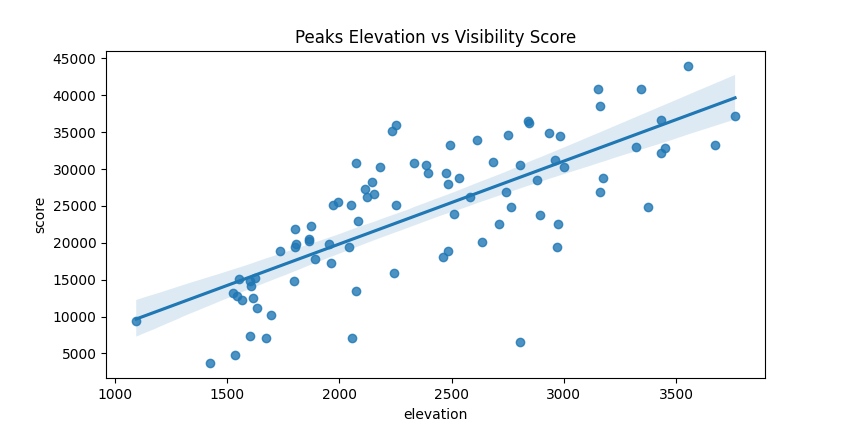
Thanks to its scalability, the aforementioned approach can be easily extended to the analysis of the visibility of routes, with the aim of finding the most panoramic ones. Given the nature of the research question, the analysis is performed exclusively on mountain trails; however, the following procedures can be extended to integrate other types of routes such as public roads.
To compute the visibility score for each route, a naive approach was followed. As emerged from the data analysis phase (Section 3), the geometries contained in the provided shapefile of the mountain trails are of type LineString. Since the application of the visibility analysis to sets of points is computed on raster data, then the conversion of the routes to a raster format is required. Therefore, a binary-valued matrix with the same dimensions of the DEM raster is computed, assigning values equal to 1 to the cells that are crossed by the routes, and 0 to the others. An example of representation of the rasterized routes is shown in Figure 9.
Once the routes are converted to a raster format, it is straightforward to apply the visibility analysis procedures described in Section 4.4. Basically, the naive approach consists in treating each cell of the raster that is crossed by at least one route as an observed peak. Afterwards, as aforementioned, a visibility matrix, and subsequently the visibility scores matrix are computed. Finally, for each route, the panorama score is defined as the sum of all the visibility scores of the cell composing such track. However, it is evident that longer routes are more likely to have a panorama score higher than shorter routes, as they occupy more cells in the raster. Due to the sparse distribution of the routes length (Section 3), it is necessary to normalize the scores on the length of the routes. The entire procedure is represented by the function compute_routes_score.
def compute_routes_score(
    dem: np.ndarray,
    routes: gpd.GeoDataFrame,
    peaks: pd.DataFrame,
    crs: str,
    transform: Callable
) -> gpd.GeoDataFrame:
    """compute_routes_score.

    Compute the panorama score for each route on a digital elevation
    model (DEM) array based on the visibility of the peaks.
    The function:
    1. rasterizes the routes geometry to match the DEM shape and
       transform;
    2. extracts the coordinates of the rasterized routes;
    3. extracts the coordinates of the peaks;
    4. computes the visibility matrix between the routes and the peaks
       using the compute_visibility_matrix function;
    5. finds the indices of the visible pairs of routes and peaks;
    6. computes the visibility scores between the visible pairs of
       routes and peaks using the compute_visibility_scores function;
    7. creates a score matrix with the visibility scores at the routes
       coordinates;
    8. computes the panorama score for each route as the sum of the
       scores along the route;
    9. computes the panorama score weighted by the route length;
    10. adds the panorama score and the panorama score weighted as
        columns to the routes GeoDataFrame;
    11. returns the routes GeoDataFrame with the panorama scores.

    :param dem: the DEM array to compute the routes score
    :type  dem: np.ndarray
    :param routes: the GeoDataFrame of the routes with their geometry
    :type  routes: gpd.GeoDataFrame
    :param peaks: the DataFrame of the peaks with their coordinates
                  and geometry
    :type  peaks: pd.DataFrame
    :param crs: the coordinate reference system of the DEM and the
                routes
    :type  crs: str
    :param transform: the transformation function to convert the
                      coordinates to longitude and latitude
    :type  transform: Callable
    :return: the routes GeoDataFrame with the panorama score and the
             panorama score weighted
    :rtype:  gpd.GeoDataFrame
    """
    rasterized = rio.features.rasterize(
        routes.geometry, out_shape=dem.shape, transform=transform, fill=0)
    routes_coords = np.transpose(np.nonzero(rasterized))
    #
    peaks_all = peaks[['row', 'col']].values
    visibility = compute_visibility_matrix(dem, routes_coords, peaks_all)
    routes_ix, peaks_ix = np.nonzero(visibility)
    rs = routes_coords[routes_ix]
    ps = peaks_all[peaks_ix]
    scores = compute_visibility_scores(rs, ps, crs, transform)
    score_matrix = np.zeros(dem.shape)
    for i, x in scores.items():
        score_matrix[i] = x
    #
    routes['panorama_score_weighted'] = 0.
    routes['panorama_score'] = 0.
    for i, row in tqdm(routes.iterrows(), total=len(routes)):
        rst = rio.features.rasterize(
            [row.geometry], out_shape=dem.shape, transform=transform, fill=0)
        score = np.sum(score_matrix[rst!=0])
        score_weighted = score/(row.geometry.length/1e3)
        routes.loc[i, 'panorama_score_weighted'] = score_weighted
        routes.loc[i, 'panorama_score'] = score
return routesThe results of the most panoramic routes are shown in Table 5 and depicted in Figure 10. In this case, the panorama score normalized on the length is not correlated with any other variable of the routes. This may indicate an unbiased estimator of the panorama score of a mountain route, although additional analyses are necessary to verify this. As aforementioned, this is a naive approach and computing the visibility for each cell of the routes may result in computationally expensive operations. Therefore, more efficient methods should be researched for aggregating the routes in a different way, in order to compute the final panorama score.
The presented work suggests a scalable modular pipeline for the visibility analysis of mountain peaks and trails. As aforementioned, the proposed visibility analysis techniques integrate naive approaches, and are based on several assumptions for simplicity. Therefore, multiple improvements can be introduced to further strengthen the approach, enhancing both the accuracy and the validation of the final results.
First, as previously mentioned in Section 4.2, the detection of mountain peaks may be further strengthened by cross-referencing local peaks inferenced from the DEM, with peaks information provided by OpenStreetMap[12]. However, the cross-referencing is advised uniquely to refine the results inferenced from the DEM, since some secondary peaks may be not referenced by OpenStreetMap.
Second, the visibility definition is based on the assumptions discussed in Section 4.3.1:
To address the first assumption, it would be sufficient to add to the observing point the height of the observer. However, the other assumptions may result more challenging to handle. A possible solution can be the integration of a corrected DEM as provided by GDAL in the gdal_viewshed program[18]. The proposed formula for a corrected DEM \(\text{DEM}_c(p_1, p_2)\) in the context of a visibility check between two points \(p_1\) and \(p_2\) is the following: \[
\text{DEM}_c(p_1, p_2) = \text{DEM} - \lambda_c \frac{d(p_1, p_2)^2}{R}
\] where \(\text{DEM}\) is the original DEM, \(\lambda_c\) is the curvature factor, \(d(p_1, p_2)\) is the distance between \(p_1\) and \(p_2\), and \(R\) is the radius of the Earth. The curvature coefficient \(\lambda_c\) is computed as: \[
\lambda_c = 1 - \theta_r
\] where \(\theta_r\) is the refraction coefficient, which varies depending on the atmospheric conditions and the wavelength. Common values for \(\theta_r\) are \(0\) for no refraction (\(\lambda_c = 1\)), \(1/7\) for visible light (\(\lambda_c = 6/7\)), \(0.25 \sim 0.325\) for radio waves (\(\lambda_c = 0.75 \sim 0.625\)), and 1 for flat earth (\(\lambda_c =
0\))[18]. Furthermore, as regards the weather conditions, an advanced approach may cross-reference with meteorological data.
Third, the panorama score of the mountain trails may integrate further improvements. For example, not only mountaintops compose the panorama of a route, but also other points of interest such as lakes, rivers or monuments. Moreover, the analysis of viewsheds may be integrated in the routes panorama computation, since they provide a complete overview of the visible area around a given point. Obviously, these analyses are more computationally expensive to undertake, since they require to apply a visibility analysis on all the surroundings.
Finally, the overall computational operations can be improved by integrating parallelization as suggested in Section 2. Also the computation of the routes visibility can be improved, as processing them point by point is a naive approach, and may result very expensive, especially with high-resolution DEMs. The visibility between two subsequent cells in the raster is likely to change by a small degree, therefore it may be possible to integrate topographical information about the routes to inference the visibility of multiple cells at the same time.
The presented work proposes a set of techniques for the analysis of the visibility among mountain peaks and trails, based on the information of a Digital Elevation Model. After a preliminary data exploring and preprocessing phase, DEM data is exploited to extract a set of mountain peaks by means of a local maximum filter. Subsequently, a Peaks Visibility Network is computed, with edges weighted based on an inverse distance score. Finally, a technique for computing the panorama score of mountain trails is proposed, where panorama is based on the visibility between the routes and peaks. The results are the rankings of the most panoramic mountaintops and mountain trails.
Several improvements are also suggested to enhance the quality and efficiency of the analysis. The proposed techniques can be used as a baseline for future research, by leveraging on its scalability.
In conclusion, if you are planning a hiking trip in Trentino and want to enjoy the best panoramic views, consider following the SAT mountain trail number E646. Nearby, you will find Punta Penia of Marmolada, which is ranked as the second-best mountaintop for visibility, according to the presented results.
The config.yaml file is intended to be used as interface with the user, in order to customize the most important parameters, and the overall workflow of the project.
env:
  # random seed for reproducibility
  seed: 50
  # true to preprocess the data and save locally
  prepare_data: true
  figures:
    # output path to save the figures
    path: ./docs/plots
    # figures default width
    width: 850

dem:
  # output path to save the DEM
  path: ./data/dem
  # true to download the DEM
  download: true
  url:
    # root url for the download
    root: https://tinitaly.pi.ingv.it
    # download endpoint
    download: Download_Area1_1.html
  # tiles to download and process (see TINITALY webpage for codes)
  tiles:
  - w51560
  - w51060
  - w50560
  - w51565
  - w51065
  - w50565
  - w51570
  - w51070
  - w50570
  # downsampling resolution in meters, original is 10 meters
  downsampling: 100 # meters
  # output path to save the processed DEM
  output: ./data/dem/trentino.tif

boundaries:
  # keyword to search for retrieving regional area from ISTAT dataset
  region: trento
  path:
    # output path to save the boundaries
    root: ./data/boundaries
    # endpoint of the shapefile to load
    shp: Limiti01012023_g/ProvCM01012023_g
  # output path to save the processed boundaries
  output: ./data/boundaries/boundaries.parquet
  # true to download the boundaries
  download: true
  # boundaries dataset url (zip file)
  url: https://www.istat.it/storage/cartografia/confini_amministrativi/generalizzati/2023/Limiti01012023_g.zip

routes:
  # routes dataset url (zip file)
  url: https://sentieri.sat.tn.it/download/sentierisat.shp.zip
  # output path to save the routes
  path: ./data/routes
  # output path to save the processed routes
  output: ./data/routes/routes.parquet
  # true to download the routes
  download: true

peaks:
  # local filter size for peak detection
  size: 50
  # elevation threshold for filtering detected peaks.
  # Retain only peaks above this threshold
threshold: 1000At the early stages of the code development, the computation of visibility algorithms was not efficient. To exploit parallelization and speed up the computations, Numba was used[19] .
Numba is an open source Just-In-Time (JIT) compiler for Python, which converts NumPy code into machine code. It can leverage vectorization and parallelization, both on the CPU and on the GPU. In this project, some functions are implemented with the @njit decorator, which allows for the generation of machine code if compatible. Some functions also exploit parallelization for better performance.
The production of this report was done with Quarto[20], which is an open-source tool for the production of both scientific and technical documents. It was employed due to his easy integration of Python and Jupyter Notebooks.